Factor Graphs

Reading notes on Dellaert & Kaess, “Factor Graphs for Robot Perception”. Source notebook: rmath/factor_graphs_dellaert_kaess.ipynb — repo not public yet.

My first exposure to SLAM was EKF and learned about cartographer during my internship at BNR over the summer. Got to know about GTSAM there while digging around the calibration stack. I mainly did the systemic error parameter calibration for the odometry. And here I was in my third semester digging into factor graphs when Im supposed to be writing a local planner for topological maps. This document is mostly my notes during that time latexised and tied to the micro lie theory notes in the other document that in turn ties to the ranif library.

This mostly covers the Dellart-Kaess paper and some references to Girisetti et al which is pretty lean but has some good block representations. In the paper they say can be used for inference problems in robotics and I have seen them try to push factor graphs for neural nets but have only seen it been used in state estimation.

Introduction

Ill skip over a lot of the stuff covered in the initial portion of the text and provide just a one liner since these are pretty much the base of any method. Eerything is probabilistic inference and how it is conveyed across the system.

$p(\mathbf{X}|\mathbf{Z})$ - the conditional densisty that gives the pose estimates given the measurements and a priori knowledge. Graphical models provide a way cleaner approach to characterize this which factorizes the high dimensional probability densities as a product of mansmaller domain probability density factors.

They state bayesian networks for generative modeling and this again is where the use of words leads to so many gaps in ones knowledge. Why is it generative?

Irrespective of what they call it, bayes net in this case is pretty useful to represent the joint density of the poses and the landmarks and the measurements observed that connect them. Below is the example straight out of the paper.

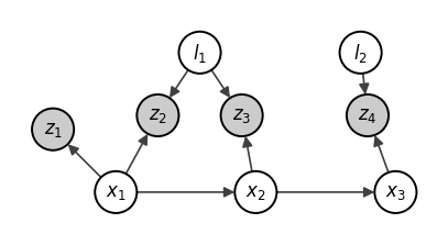
For this example the joint density $p(\mathbf{X}|\mathbf{Z}) = p(x_1, x_2, x_3, l_1, l_2, z_1, z_2, z_3, z_4)$ which is the product of the conditional densities:

The lines differentiate clearly the various kinds of information that is available and used to setup the joint densities using the conditional densities of the markov chain on the pose, prior density, conditional density on the absolute pose, measurement model condition densities.

Ive always wodered if the associations can be modeled as a distribution itself. I think I remember maybe in optimus ride where I had encountered a paper that did this. Will have to find it somewhere

Everything is assumed to be multivariate gaussian distribution for each of the densities mentioned above. Have additonal processing to mitigate the non linearity in these models.

In the introduction there is one section that is dedicated for simulating from the bayes net model, which makes very little sense though unless they mean that they are characterizing the actual environment and behavior using this model. Irrespective of whether we are “simulating” or modeling the process or rather the state from a bayes net it is easier to get the estimate which they call as simulate by doing a topological sort and then estimate them in subsets rather than doing a joint updation on the entire system.

Two important terminologies that feel similar and are very much intertwined are the posterior and likelihood. From the bayesnet we are maximizing a posterior to get the unknown variables X i.e. 

The normalizing factor $p(\mathbf{Z})$ doesnt really matter and it just boils down to the likelihood of the states X given the measurements Z. The likelihood is esssentially a function in $X$ with $Z$ as the parameters. How well conditioned is $X$ tells whther we can find a solution or not and well conditioned in this sense is how many parameters of $Z$ provide good constraints on $X$

This demarcation between the measurements and the states calls for a different graphical model and these guys at least thats what I think introduce factor graphs. since I havent specifically seen the modeling portion using bayes net, Ive only used filtering using EKF or factor graphs so I specifically havent used bayes nets, which is now worth exploring atleast to take a look at how they are actually used.

The above bayes net becomes the following MAP equation for the toy example:

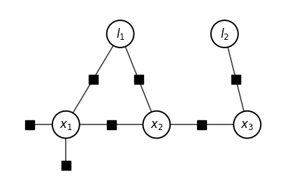
Note that there is an additional node associated with $x_1$ and there is a specific node connecting the conditional density between each state nodes as well. The paper states that unlike in bayes net there is no explicit measurement node specified, but rather than an explicit measurement node there are additional explicit nodes representing this information and even the implied markov chains that are represented by the edges are spelled out using factor nodes connecting those state nodes.

As a formal definition factor graph is a bipartate graph $F= (U, V, E)$ with two types of nodes: factors $\phi \in U$ and variables $x_j \in V$. Edges $e_{ij} \in E$ are between factors and variable nodes. And then theres one set which has all the variable nodes adjecent to a factor $\phi_i$ that is written as $N(\phi_i)$ and that is written as $X_i$. Factor graph $F$ defines the factorization of a global function $\phi(X)$ as

Each of the constraints are independent condition desnsities. These are provided by the edges $e_{ij}$ with the factor $\phi_i$ containing only the variables $X_i$ that are in the adjacency set $\mathcal{N}(\phi_i)$

Converting bayes net to factor graph: 1. every bayes net node splits into both the variable node and the factor node. 2. factor node is connected to variable node from which it was extracted from along with the parent node that this associated to. 3. If some nodes are measurement evidence node then they just become parameters in the factor node.

The final form of the toy example in correct factor graph factorization:

Some comments in this section worth mentioning: 1. Evaluating this function is easy once the factor graph is properly generated. 2. Easier to work in log or negative log space obviously. 3. All gradient agnostic methods can be used to optimize da we have a cost function to optimize 4. a. Much easier if it is continuous and gradient based methods can make it quick. b. discrete variables - graph search methods which are expensive 5. Generally its always a mixture of the two

Have to define the variants somewhere and represent them as factor graphs and then apply it. My theoritical curiosity(which is only a curiosity and hasnt got anywhere).

Have to checkout Gibbs sampling, have never used it anywhere.

Smoothing and Mapping

Given that we have a number of factors that are mostly non-linear the objective of SLAM is to find the values that maximally agree to the constraints these factors or rather the uncertain measurements which are called as factors define. not spelling out each and every specific thing out here.

MAP inference:

We had

Assuming that all the factors are gaussians with zero mean noise

Contains both the gaussian priors and likelihood factors.

Changing to negatve log space and dropping the constant finding the MAP becomes a minimization problem of the following:

Often as is the case of the sensors we have the measurements are normally of a lower dimension than the unnown $X_i$ we are computing and naturally there are a lot more solutions that satisfy the constraint. So we need multiple measurements adding to the constraints in order to extract a unique solution of the variables.

The crux of everything now is, since $h_i$ is non linear we would need a good initial estimate and from there non-linear optimizations like Gauss-Newton and LM can be applied. Any non linear optimization is just iteratively reducing the cost by linearizing and moving towards tha global minimum.

Taylor’s expansion, here it comes. Linearizing $h(\cdot)$ in the least quares objective function:

and the measurement jacobian $H_i$ is the multivariate partial derivative of $h_i$ at a given linearization point $X^0_i$,

and $\Delta_i \defeq X_i - X^0_i$ is the state update vector. Relating these to the Lie group treatment, $H_i$ is essentially the tangent space at the measurement point which is ${}^X\tau$ when the state space is a manifold.

Now substituting the linearization in the cost function:

where $z_i - h_i(X^0_i)$ is the prediction error at the linearization point. Note the clean tying to bayes filters

The scaling of the entire error function can be re-written by changing the variables.

and substituting the error function:

This is called whitening which eliminates the units all together as well and allows for different kinds of measurements to contribute to the cost function.

Final form:

Once this least squares function is established its a number of different factorizations to solve for $\Delta^*$ which is full rank $m \times n$ matrix $A$ with $m \geq n$.

• Cholesky: positive definite, factored using the information matrix $\Lambda \defeq A^\top A = R^\top R$
• QR: more accurate, more stable, directly factorizes $A$. Slower than cholesky.

One big thing to notes is sparsity which allows for some better tricks to use.

Optimization algorithms: - Stepest descent - direction of the jacobian - Guass-Newton - direction of the hessian - LM - alternate between jacobian and hessian - Dogleg method - pre-compute both and use whichever is valid in that step

Sparsity

Not everything is connected to everything so the jacobian matrix A that is setup is actually very sparse that allows for some tricks that help in reducing the complexity of the factorizations required to find the $\Delta$ in each step of the optimization.

Refering back to the factors in the equation for the toy example

the block structure of the sparse jacobian is

The information matrix $\Lambda = A^\top A$ is what Cholesky actually factors. Writing it down by hand below:

Asked claude to write it in SymPy which I found out about. Pretty neat imho

import sympy as sp

cols = ['l1', 'l2', 'x1', 'x2', 'x3']

# the sparsity spec straight from [A|b]: (row, col) pairs that carry a nonzero A_ij.
# rows are the factors phi_1..phi_9 (1-indexed), cols are 1..5 as above.
nz = [(1, 3), (2, 3), (2, 4), (3, 4), (3, 5),
      (4, 1), (5, 2), (6, 3),
      (7, 1), (7, 3), (8, 1), (8, 4), (9, 2), (9, 5)]

# build A as a 9x5 matrix: each nonzero is its own symbol A_{ij}, everything else 0.
A = sp.zeros(9, 5)
for (i, j) in nz:
    A[i - 1, j - 1] = sp.Symbol(f'A{i}{j}')   # A.row/col are 0-indexed, symbol name keeps 1-index

Lambda = sp.simplify(A.T * A)   # the 5x5 information matrix  A^T A

# pretty-print with the variable names on the axes
sp.Matrix(Lambda)

$\displaystyle \left[\begin{matrix}A_{41}^{2} + A_{71}^{2} + A_{81}^{2} & 0 & A_{71} A_{73} & A_{81} A_{84} & 0\\0 & A_{52}^{2} + A_{92}^{2} & 0 & 0 & A_{92} A_{95}\\A_{71} A_{73} & 0 & A_{13}^{2} + A_{23}^{2} + A_{63}^{2} + A_{73}^{2} & A_{23} A_{24} & 0\\A_{81} A_{84} & 0 & A_{23} A_{24} & A_{24}^{2} + A_{34}^{2} + A_{84}^{2} & A_{34} A_{35}\\0 & A_{92} A_{95} & 0 & A_{34} A_{35} & A_{35}^{2} + A_{95}^{2}\end{matrix}\right]$

Rewriting the above as just the information matrix symbols:

This is exactly of the form that one would get when the SLAM toy example is represented using yet another graphical model MRF. The hessian $\Lambda = A^{\top}A$ and the adjacency matrix $G$ of an MRF are one and the same. I had always viewed MRF in a different light and this links even factor graphs and MRF in SLAM.

The authors mention a different route in which $\lVert A\Delta - b \rVert_2^2$ is expanded and this gives rise to a different form that is directly linked to the densities induced by binary MRFs. That portion introduces yet another set of symbols that Im particulary not amused by and am just skipping it altogether